Spectral 2-D Navier–Stokes solver — Kelvin–Helmholtz Instability#
This demo solves the incompressible 2-D Navier–Stokes equations on a
periodic rectangular domain using a pseudo-spectral method with a
semi-implicit time integrator. The simulation is initialised with the
smooth shear-layer profile proposed by McNally, Lyra & Passy (2012) as a
well-posed benchmark for the Kelvin–Helmholtz instability (KHI). Vorticity
snapshots are written at regular intervals using the tecio Python API for
animation in Tecplot 360.
1. Governing equations#
The incompressible Navier–Stokes equations in 2-D are
where \(u_i = (u, v)^T\) is the velocity vector, \(p\) is kinematic pressure (pressure divided by density), \(\nu\) is kinematic viscosity, and \(f_i\) is an optional external body force.
The convective term is written in divergence form \(\partial(u_i u_j)/\partial x_j\) rather than advective form \(u_j \partial u_i/\partial x_j\). The two are equivalent under incompressibility:
The divergence form is preferred here because the products \(u_i u_j\) can be computed directly in physical space and then transformed to spectral space (see Section 2).
The incompressibility constraint couples the pressure to the velocity through a Poisson equation obtained by taking the divergence of the momentum equation:
After each momentum update the velocity is projected onto the divergence-free subspace by subtracting the pressure gradient:
Component form#
Writing out both momentum equations explicitly with the body force retained (used in the alternating-jet variant of this script):
2. Pseudo-spectral discretisation#
Fourier representation#
On a periodic domain of width \(L_x\) and height \(L_y\), any field \(q(x,y)\) can be represented by its 2-D discrete Fourier transform:
with corresponding wavenumbers
In spectral space, spatial derivatives become algebraic multiplications:
Spectral Laplacian#
The scalar Laplacian in spectral space is therefore
stored in the array lap in the code (\(\lambda \leq 0\)). The
zero-wavenumber mode is set to \(1\) to avoid division by zero; the mean
pressure is enforced separately.
Nonlinear convection — pseudo-spectral approach#
The convective fluxes \(u_i u_j\) are computed in physical space (pointwise multiplications) and then transformed to spectral space, where the outer derivative becomes a wavenumber multiplication:
giving the spectral convective terms for each momentum equation:
3. Time integration — IMEX semi-implicit scheme#
Convection and forcing are treated explicitly (forward Euler) while diffusion is treated implicitly with a Crank–Nicolson average, averaging the diffusion operator between levels \(n\) and \(n{+}1\). This avoids the parabolic stability constraint \(\Delta t \leq \Delta x^2/(2\nu)\) while keeping the nonlinear term cheap to evaluate. The semi-discrete equations in spectral space are:
where \(\lambda = (\mathrm{i}k_x)^2 + (\mathrm{i}k_y)^2 \leq 0\) is the spectral Laplacian eigenvalue. Collecting \(\hat{u}^{\,n+1}\) on the left and solving gives the explicit update rules:
Because \(\lambda \leq 0\) the denominator is strictly positive for all wavenumbers, giving unconditional stability for the diffusive modes. In code (with forcing absent for the KHI case):
u_hat = (u_hat*(1/dt + nu*lap) - conv_u + fx)/(1/dt - nu*lap)
v_hat = (v_hat*(1/dt + nu*lap) - conv_v + fy)/(1/dt - nu*lap)
Adaptive CFL time step#
The time step is set by the advective CFL condition:
with a small regularisation \(\varepsilon = 10^{-8}\) added to \(|\mathbf{u}|_{\max}\) to handle the zero-velocity initial condition.
4. Pressure projection#
The velocity field \(\hat{u}_i^*\) produced by the momentum update is not yet divergence-free. Taking the divergence of the momentum equation and invoking the incompressibility constraint \(\partial u_j^{n+1}/\partial x_j = 0\) gives the Poisson equation for pressure in spectral space:
The mean pressure \(\hat{p}_{00} = 0\) is enforced explicitly. The velocity is then corrected by subtracting the spectral pressure gradient:
This standard projection step enforces incompressibility at each time level.
5. Vorticity diagnostic#
The scalar vorticity \(\omega = \partial v/\partial x - \partial u/\partial y\) is computed without any finite-difference approximation:
and recovered in physical space via a single inverse FFT.
6. Kelvin–Helmholtz initial conditions#
The KHI initial condition follows the smooth shear-layer profile of McNally, Lyra & Passy (2012) (ApJS 201, 18), which is designed to be well-posed and support convergent simulations. A piecewise-exponential profile is used to approximate a hyperbolic-tangent shear layer while remaining periodic on the unit square \([0,1]^2\):
with \(U_1 = 0.5\), \(U_2 = -0.5\), and layer thickness \(L = 0.025\). Two counter-flowing shear layers are present (at \(y = 1/4\) and \(y = 3/4\)), consistent with the periodic domain. A small sinusoidal perturbation seeds the instability:
A passive tracer \(\phi\) is initialised to \(1\) in the inner jet region (\(1/4 \leq y < 3/4\)) and \(0\) in the outer streams, approximating a colour dye placed in the fluid to trace the density interface typically visualised in KHI problems. The tracer satisfies the pure advection equation:
which is solved by semi-Lagrangian advection — each grid point is traced backward one step along the velocity field and \(\phi\) is interpolated there:
ix = (X - u * dt_out) / dx % nx
iy = (Y - v * dt_out) / dy % ny

phi = map_coordinates(phi, [ix.ravel(), iy.ravel()],
                      order=1, mode='wrap').reshape(nx, ny)
The key motivation for this smooth profile is that a sharp (discontinuous) shear layer does not converge with grid refinement — numerical noise seeds structure at all scales. With the smooth exponential profile, the dominant instability mode is set by the physical shear-layer thickness \(L\) rather than the grid spacing.
7. Simulation parameters#
Parameter |
Symbol |
Value |
|---|---|---|
Domain size |
\(L_x \times L_y\) |
\(1.0 \times 1.0\) |
Kinematic viscosity |
\(\nu\) |
\(3.675 \times 10^{-5}\) |
Background velocities |
\(U_1,\,U_2\) |
\(+0.5,\,-0.5\) |
Shear-layer thickness |
\(L\) |
\(0.025\) |
Perturbation amplitude |
— |
\(0.01\) |
Output interval |
— |
\(\Delta t_\text{out} = 0.01\) |
End time |
\(T\) |
\(15.0\) |
Resolution-dependent CFL factors#
Balancing instability growth against numerical stability required adjusting the CFL factor with resolution (see Section 8):
Grid |
\(N_x \times N_y\) |
CFL |
|---|---|---|
Low |
\(256 \times 256\) |
\(0.10\) |
Medium |
\(512 \times 512\) |
\(0.15\) |
High |
\(1024 \times 1024\) |
\(0.30\) |
8. Resolution effects and numerical stability#
Balancing physical instability against diffusion#
For the KHI to develop and roll up into billows, the viscous damping time must be long compared to the instability growth time. The characteristic linear growth rate scales as \(\sigma \sim U_1/(2L)\), while viscosity damps structures of scale \(\ell\) over a time \(\tau_\nu \sim \ell^2/\nu\). A lower viscosity promotes instability growth but reduces the effective resolution of the flow, increasing the risk of aliasing and spectral blocking at the grid scale.
The value \(\nu = 3.675 \times 10^{-5}\) was chosen as a compromise: low enough that the KHI billows grow and roll up before diffusion damps the shear layer, but large enough to damp energy accumulating at high wavenumbers and prevent the simulation from blowing up.
CFL and the semi-implicit time step#
Because the diffusion term is treated implicitly, the time step is constrained only by the advective CFL condition. However, at high resolution the spectral method resolves shorter wavelengths whose phase errors accumulate more rapidly. A more conservative CFL is therefore required at low resolution to prevent the explicit convection scheme from becoming unstable — counter-intuitively, the coarser grids use the smaller CFL. At high resolution the flow is smoother (diffusion is more effective relative to the grid scale) and a larger CFL is stable.
Grid-scale instabilities at low resolution#
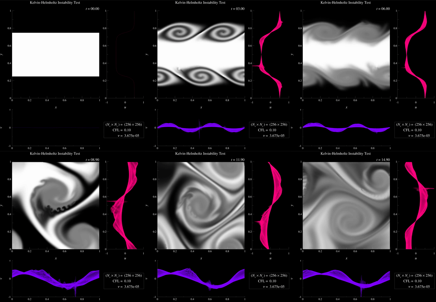
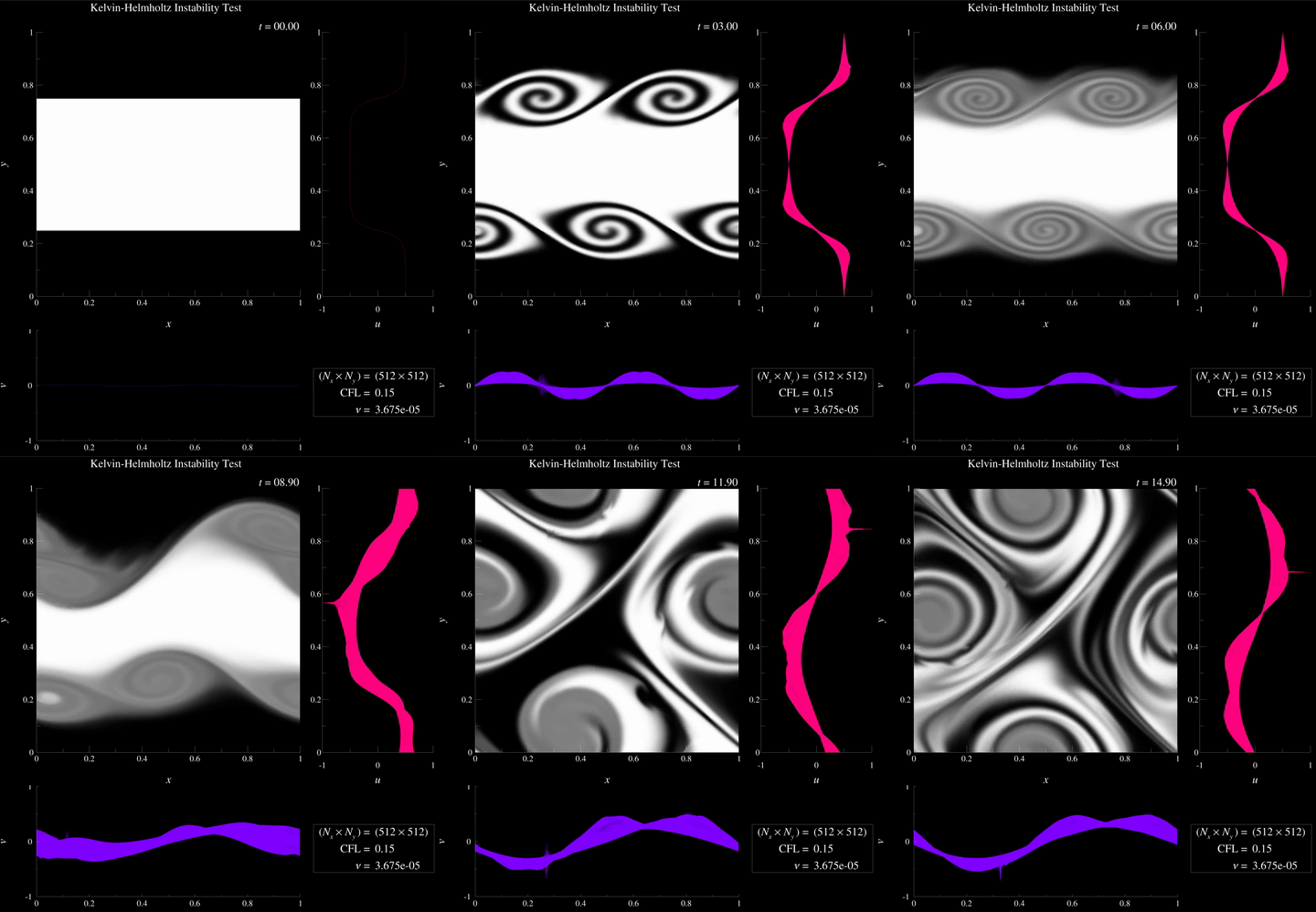
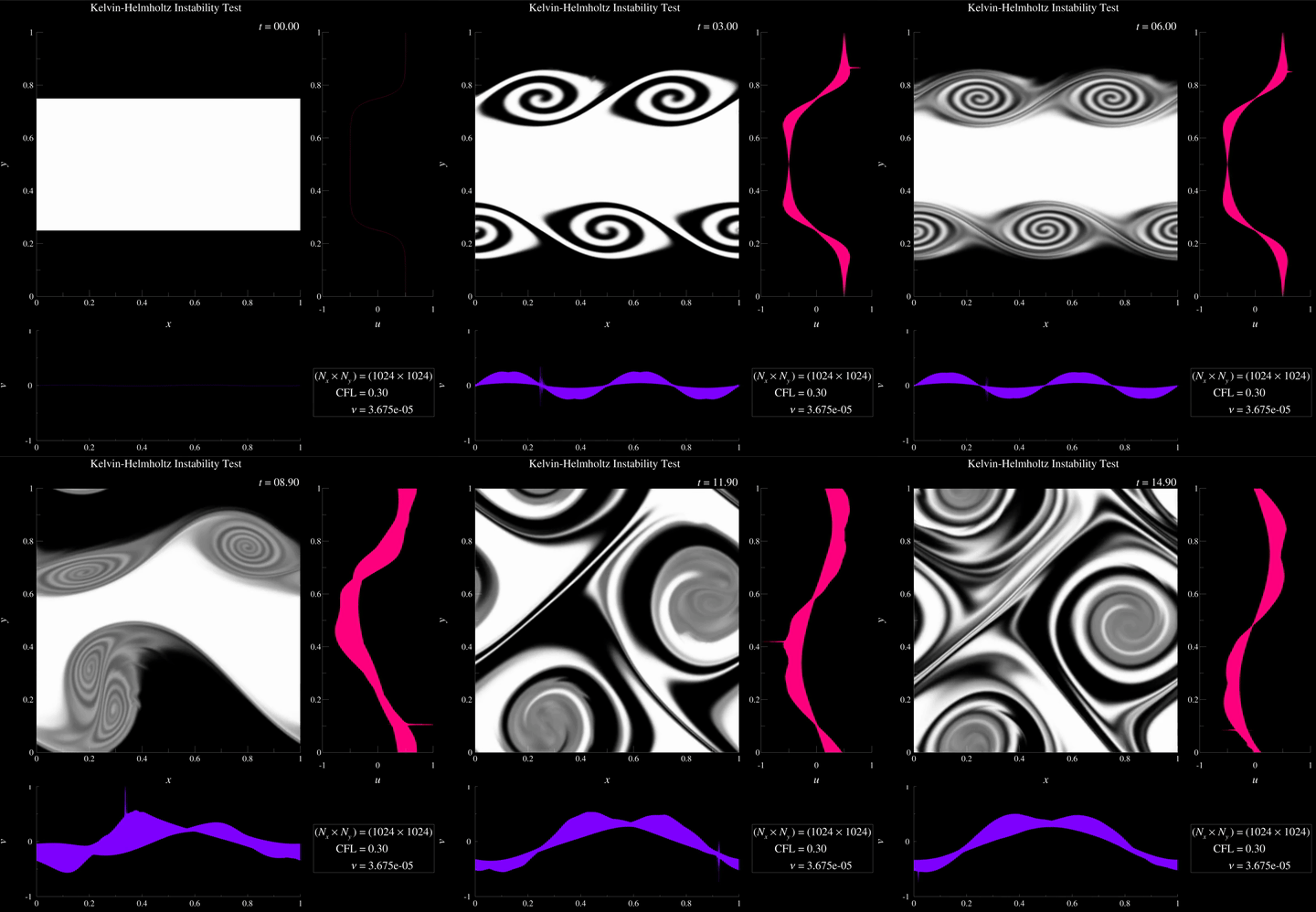
At \(256 \times 256\) the spectral resolution is marginal for the chosen parameters. Odd–even, grid-point-to-grid-point oscillations appear in the vorticity field — a classic spectral aliasing artefact. Because the pseudo-spectral method computes nonlinear products in physical space and then transforms back, the quadratic terms fold energy from wavenumbers above the Nyquist limit back into the resolved range. When viscous dissipation is insufficient to drain this aliased energy, it accumulates at the grid scale and manifests as the characteristic “salt-and-pepper” noise visible in the low-resolution animations. Increasing the grid to \(512 \times 512\) or \(1024 \times 1024\) substantially suppresses this artefact: the additional resolved modes push the aliasing to higher wavenumbers where viscosity is more effective.
9. Writing time-dependent data with tecio#
The simulation outputs a flow-field snapshot every WRITE_INTERVAL steps.
The file is opened once and each snapshot is appended as a new zone. Dataset-level
auxiliary data is written once at the start to record simulation parameters and
hint Tecplot which variables to use for axes and velocity components:
with tecio.open("simple_spectral2.szplt", "w") as szl:
    szl.add_auxdataset_dict({
        "Common.XVar": 1,
        "Common.YVar": 2,
        "Common.UVar": 3,
        "Common.VVar": 4,
        "Common.CVar": 9,
        "Nx": nx,
        "Ny": ny,
        "CFL": cfl,
        "Viscosity": nu,
        "U1": U1,
        "U2": U2,
        "L": L,
    })
The Common.* keys are recognised by Tecplot 360 and automatically configure
the spatial axes and velocity vectors on load. Common.CVar sets the default
contour variable on load, here setitng to the variable number containing the
flow tracer. The remaining keys are available as scalars for use in dynamic
text or equations
Save memory by writing coordinate arrays only once#
For the very first output frame (szl.current_zone == 0) the coordinate
arrays X and Y are written alongside the solution fields. All
subsequent zones share those arrays from zone 1 and supply only the
updated solution data:
szl.write_ijk_zone(
    title=f"Flow Field Step {k}",
    variables=["x", "y", "uvel", "vvel", "pres", "vort", "div", "qcrit", "tracer"],
    data=[X, Y, *flow] if szl.current_zone == 0 else flow,
    var_sharing=None if szl.current_zone == 0 else [1, 1] + [0] * len(flow),
    strand_id=1,
    solution_time=t,
    aux={"dt": dt, "SubIterCount": count},
)
The var_sharing list maps each variable slot to the 1-based zone index it
should be copied from; a value of 0 means the variable is supplied
directly. For a \(1024 \times 1024\) grid saved at 150 output times, sharing
the coordinate arrays avoids writing roughly
\(150 \times 2 \times 1024^2 \times 4\ \text{bytes} \approx 1.3\ \text{GB}\)
of redundant data.
10. Animate results with Tecplot#
To generate the animation from the .szplt output, run the provided macro in
batch mode:
$ tec360 -b simple_spectral.mcr
Results at three resolutions — note the progressive suppression of grid-scale noise and the increasingly well-defined vortex cores as resolution increases:
References#
McNally, C. P., Lyra, W., & Passy, J.-C. (2012). A Well-posed Kelvin–Helmholtz Instability Test and Comparison. ApJS, 201, 18. doi:10.1088/0067-0049/201/2/18