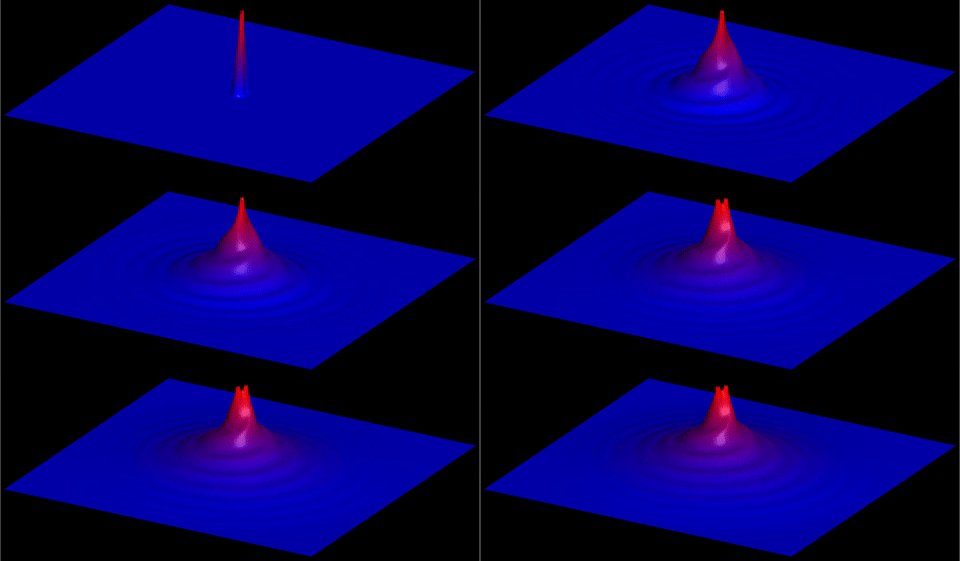
Gravity wave animation around binary black holes#

This demo simulates a scalar wave field on a 2D grid driven by a pair of orbiting point-mass sources, then writes time-dependent structured-grid data using the tecio Python API for visualization and animation in Tecplot 360.

1. Physical model#

We solve the scalar wave equation with a gravitational potential source term on a uniform 2-D Cartesian domain \(\Omega = [-1,1]^2\):

\[ \frac{\partial^2 \phi}{\partial t^2} = c^2 \nabla^2 \phi + S(\mathbf{x}, t) \]

where \(\phi(\mathbf{x},t)\) is the scalar wave field, \(c\) is the wave speed, and \(S\) acts as a forcing/constraint derived from the Newtonian potential of two orbiting masses.

Gravitational potential#

Two point masses \(M_1\) and \(M_2\) orbit their common centre of mass in a circular binary with angular frequency \(\omega\) and separation radius \(r_0\):

\[ x_p(t) = r_0 \sin(2\pi\omega t), \qquad y_p(t) = r_0 \cos(2\pi\omega t) \]

The combined Newtonian potential seen at grid point \((x, y)\) is

\[ \Phi(x, y, t) = \frac{G M_1}{\sqrt{(x_p - x)^2 + (y_p - y)^2}} + \frac{G M_2}{\sqrt{(-x_p - x)^2 + (-y_p - y)^2}} \]

Grid cells where \(\Phi > c^2\) are treated as inside the “black-hole” horizon and are pinned to \(-c^2\), mimicking an absorbing interior boundary.

2. Numerical discretisation#

Spatial grid#

The domain is discretised on an \(M \times N = 401 \times 401\) uniform grid with equal spacing in both directions:

\[ \Delta x = \Delta y = \frac{2}{M - 1} \]

Time stepping — explicit leap-frog#

Three consecutive time levels are stored in f[:, :, 0:3] (past, present, future). The update rule for interior nodes is the standard second-order centred finite difference applied to the wave equation:

\[ \phi^{n+1}_{i,j} = 2\phi^n_{i,j} - \phi^{n-1}_{i,j} + c^2 \frac{\Delta t^2}{\Delta x^2} \left( \phi^n_{i-1,j} + \phi^n_{i+1,j} + \phi^n_{i,j-1} + \phi^n_{i,j+1} - 4\phi^n_{i,j} \right) \]

The Courant–Friedrichs–Lewy (CFL) stability condition for a 2-D scalar wave equation is

\[ \Delta t \leq \frac{\Delta x}{c\sqrt{2}} \]

The simulation uses \(\Delta t = 0.125\,\Delta x / c\), which is safely below this limit.

Absorbing boundary layer#

Reflections from the domain edges are suppressed by multiplying the entire field by a spatially varying absorption mask \(\alpha(r)\) at every time step:

\[\begin{split} \alpha(r) = \begin{cases} 1 & r < 0.8 \\ \dfrac{(0.8)^n}{r^n} & r \geq 0.8 \end{cases} \quad \text{with } n = 0.045,\ r = \sqrt{x^2 + y^2} \end{split}\]

This smoothly damps outgoing waves before they reach the grid boundary.

Jacobi smoothing#

Every write_interval steps a single Jacobi iteration is applied to both the current and previous time levels to suppress high-frequency grid-scale noise:

\[ \phi^n_{i,j} \leftarrow \tfrac{1}{4} \left( \phi^n_{i-1,j} + \phi^n_{i+1,j} + \phi^n_{i,j-1} + \phi^n_{i,j+1} \right) \]

3. Simulation parameters#

Parameter	Symbol	Value
Grid size	\(M \times N\)	\(401 \times 401\)
Wave speed	\(c\)	\(1.0\)
Gravitational constant	\(G\)	\(0.01\)
Masses	\(M_1, M_2\)	\(1.0\)
Orbit radius	\(r_0\)	\(0.025\)
Orbit frequency	\(\omega\)	\(4.0\)
Time step	\(\Delta t\)	\(0.125\,\Delta x / c\)
End time	\(t_\text{end}\)	\(10.0\)

4. Writing time-dependent data with `tecio`#

The tecio library provides a Python context-manager interface for writing Tecplot SZL (.szplt) files. The file is opened once and each output frame is appended as a new ordered (IJK) zone assigned to a Tecplot strand, which is the mechanism Tecplot uses to animate data over time.

import tecio

with tecio.open("gravity_waves.szplt", "w") as szl:
    ...

Save memory by writing coordinate arrays only once#

For the very first output frame (szl.current_zone == 0) the coordinate arrays X and Y are written alongside the solution field phi, but are shared from zone 1 for all subsequent arrays. This can be done cleanly from within the zone writing call as:

szl.write_ijk_zone(
    title="Wave Field",
    variables=["x", "y", "phi"],
    data=[X, Y, f[:, :, 2]] if szl.current_zone == 0 else [f[:, :, 2]],
    var_sharing=None if szl.current_zone == 0 else [1, 1, 0],
    strand_id=1,
    solution_time=t,
)

Variable sharing avoids storing redundant coordinate data for every time step — for a 401×401 grid over hundreds of frames this reduces the output file size significantly.

Strand and solution time#

Setting strand_id=1 and incrementing solution_time tells Tecplot that all zones belong to the same time-dependent dataset. Tecplot’s animation engine will then step through the zones in solution-time order, producing a smooth animation of the evolving wave field.

5. Animate results with Tecplot#

To generate the included animation, run the provided macro in batch mode:

$ tec360 -b gravity_waves.mcr

Final result:

gravity-waves-demo

Gravity wave animation around binary black holes

On this page