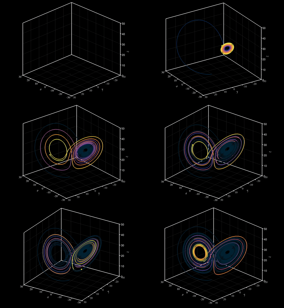
Lorenz attractor animation#

This demo generates a Lorenz attractor using classical RK4 numerical integration, then writes both a static reference trajectory and a time-dependent animated dataset using the tecio Python API for visualization in Tecplot 360.

1. The Lorenz system#

The Lorenz system is a set of three coupled, nonlinear ordinary differential equations that exhibit sensitive dependence on initial conditions — a hallmark of deterministic chaos.

The equations are:

\[ \frac{dx}{dt} = \sigma (y - x) \]

\[ \frac{dy}{dt} = x(\rho - z) - y \]

\[ \frac{dz}{dt} = xy - \beta z \]

where the three parameters control the character of the flow:

Parameter	Symbol	Value	Physical meaning
Prandtl number	\(\sigma\)	\(10\)	Ratio of momentum to thermal diffusivity
Rayleigh number	\(\rho\)	\(28\)	Normalised temperature difference driving convection
Geometric factor	\(\beta\)	\(8/3\)	Aspect ratio of the convection rolls

At these classical values the system exhibits chaotic behaviour, and trajectories converge onto the iconic two-lobed strange attractor with fractal dimension \(\approx 2.06\).

import numpy as np

sigma = 10.0
beta  = 8.0 / 3.0
rho   = 28.0

def lorenz(state):
    x, y, z = state
    dx = sigma * (y - x)
    dy = x * (rho - z) - y
    dz = x * y - beta * z
    return np.array([dx, dy, dz])

2. Numerical integration — classical RK4#

We integrate the system using the classical fourth-order Runge–Kutta method. Given the state vector \(\mathbf{u}^n = (x, y, z)^T\) at time \(t_n\), the update to \(t_{n+1} = t_n + \Delta t\) is

\[ \mathbf{u}^{n+1} = \mathbf{u}^n + \frac{\Delta t}{6}\left(\mathbf{k}_1 + 2\mathbf{k}_2 + 2\mathbf{k}_3 + \mathbf{k}_4\right) \]

where the four stage derivatives are

\[\begin{split} \begin{aligned} \mathbf{k}_1 &= f\!\left(\mathbf{u}^n\right) \\ \mathbf{k}_2 &= f\!\left(\mathbf{u}^n + \tfrac{\Delta t}{2}\,\mathbf{k}_1\right) \\ \mathbf{k}_3 &= f\!\left(\mathbf{u}^n + \tfrac{\Delta t}{2}\,\mathbf{k}_2\right) \\ \mathbf{k}_4 &= f\!\left(\mathbf{u}^n + \Delta t\,\mathbf{k}_3\right) \end{aligned} \end{split}\]

and \(f(\mathbf{u})\) is the right-hand side of the Lorenz system above.

RK4 has a local truncation error of \(\mathcal{O}(\Delta t^5)\) and a global error of \(\mathcal{O}(\Delta t^4)\), making it an excellent balance of accuracy and cost for smooth ODE systems. The simulation uses \(\Delta t = 0.01\) over \(5000\) steps, giving a total integration time of \(T = 50\).

dt      = 0.01
n_steps = 5000

traj  = np.zeros((n_steps, 3))
state = np.array([1.0, 1.0, 1.0])

for i in range(n_steps):
    traj[i] = state

    k1 = lorenz(state)
    k2 = lorenz(state + 0.5 * dt * k1)
    k3 = lorenz(state + 0.5 * dt * k2)
    k4 = lorenz(state + dt * k3)

    state = state + (dt / 6.0) * (k1 + 2*k2 + 2*k3 + k4)

The full trajectory is stored row-wise in traj and then split into coordinate arrays:

x = traj[:, 0]
y = traj[:, 1]
z = traj[:, 2]

3. Additional variables — \(t\) and \(\tau\)#

Two scalar variables are written alongside the spatial coordinates:

\(t\) — the absolute simulation time at each point along the trajectory, \(t_i = i \,\Delta t\). For the growing-trajectory animation this allows Tecplot to colour the curve by age.
\(\tau\) — the time relative to the current frame, defined as \(\tau_i = (i - i_\text{frame}) \,\Delta t \leq 0\). This gives every point a value of zero at the head of the curve and increasingly negative values further back along the tail, which is useful for applying a fade effect in the colour map.

For the static reference zone and the moving particle, \(t\) and \(\tau\) are declared passive — they occupy a slot in the variable list but no data is stored or written for them, saving memory and file space.

4. Writing time-dependent data with `tecio`#

The tecio library exposes a Python context-manager interface for writing Tecplot SZL (.szplt) files. All zones are appended to a single open file handle within the with block.

import tecio

with tecio.open("lorenz.szplt", "w") as szl:
    ...

Static reference zone (strand 0)#

The complete attractor is written as a single ordered (IJK) line zone with \(I = N_\text{steps}\), \(J = K = 1\). Setting strand_id=0 marks it as a static zone that is always visible regardless of the current animation time. Variables t and tau are declared passive so no data array needs to be supplied for them:

szl.write_ijk_zone(
    title="Lorenz Attractor",
    variables=["x", "y", "z", "t", "tau"],
    data=[x, y, z],
    passive_vars=[False, False, False, True, True],
    strand_id=0,
)

Growing trajectory (strand 1)#

Each frame writes the trajectory from the start up to step \(i\), so the curve grows as the animation advances. The zone at frame \(i\) contains \(i + 1\) points, giving it dimensions \((i+1, 1, 1)\):

for i in range(0, n_steps, 10):
    szl.write_ijk_zone(
        title="Trajectory",
        variables=["x", "y", "z", "t", "tau"],
        data=[
            x[:i+1],
            y[:i+1],
            z[:i+1],
            np.arange(i+1) * dt,           # t  = absolute time
            (np.arange(i+1) - i - 1) * dt, # tau = time relative to head
        ],
        strand_id=1,
        solution_time=i * dt,
    )

Assigning strand_id=1 and a monotonically increasing solution_time tells Tecplot that all these zones form a single time-evolving object. The animation engine steps through them in solution-time order.

Moving particle (strand 2)#

A second strand contains only the single point at step \(i\), creating a marker that travels along the attractor in lockstep with the growing curve. Again t and tau are passive since a single-point zone makes relative time meaningless:

for i in range(0, n_steps, 10):
    szl.write_ijk_zone(
        title="Particle",
        variables=["x", "y", "z", "t", "tau"],
        data=[x[i:i+1], y[i:i+1], z[i:i+1]],
        passive_vars=[False, False, False, True, True],
        strand_id=2,
        solution_time=i * dt,
    )

Because strands 1 and 2 share the same solution_time values, Tecplot advances both simultaneously during playback, keeping the particle exactly at the head of the growing curve.

5. Create the animation with Tecplot#

To generate the included animation, run the provided macro in batch mode:

$ tec360 -b lorenz.mcr

Final result:

lorenz-demo

Lorenz attractor animation

On this page