Quickstart#
This page introduces the tecio API with four self-contained examples. For
installation and system requirements see Installation.
Examples#
1. Structured IJK Zone (1-D Line)#
The simplest possible file: a single ordered zone containing two variables
plotted against each other as a line. Dimensions are inferred from the array
shape — a 1-D array of length N produces an (N, 1, 1) zone.
import numpy as np
import tecio

x = np.linspace(0.0, 2.0 * np.pi, 256)
y = np.sin(x)

with tecio.open("line.szplt", "w", title="Sine Curve") as w:
    w.write_ordered_zone(
        title="sin(x)",
        variables=["x", "y"],
        data=[x, y],
    )
Reading the file back follows the same pattern:
with tecio.open("line.szplt", "r") as r:
    print(r.title)  # 'Sine Curve'
    print(r.variables)  # ['x', 'y']

    zone = r.zones[0]
    x_read = zone.variables[0].values  # NumPy array, shape (256, 1, 1)
    y_read = zone.variables[1].values
Note
The tecio Python API is 0-indexed. zones and variables start at 0,
and zone_index/var_index properties, and every function or method
parameter that takes a zone or variable index all use standard Python
(zero-based) indexing: r.zones[0] is the first zone, zone.variables[1] is
the second variable.
Tecplot 360 zone and variable numbers start at one. tecio converts between the
two conventions automatically when a file is opened for reading or writing, so
a zone shown as “Zone 1” in Tecplot 360 is r.zones[0] here, and the first
variable in a .dat file’s VARIABLES = "x", "y" line is
zone.variables[0]. See Indexing Conventions for
mre information.
2. Unstructured Finite-Element Zones#
All five simple finite-element cell types supported by Tecplot are shown below
in a single file, one zone per element type. The node_map argument is a
(num_cells, nodes_per_cell) integer array of zero-based node indices,
each one an index into that zone’s coordinate arrays.
import numpy as np
import tecio
from tecio.libtecio import ZoneType

with tecio.open("fe_cells.szplt", "w") as szlfile:
    # -- Write a FE line segment ---------------------------------------------
    x = np.array([0, 0.5, 1])
    y = np.array([0, 1, 0])
    nodes = np.array([[0, 1], [1, 2]])
    c = np.sin(2 * np.pi * x) * np.cos(2 * np.pi * y)

    szlfile.write_fe_zone(
        zone_type=ZoneType.FELINESEG,
        data=[x, y, c],
        node_map=nodes,
        title="FE_LineSeg",
        variables=["x", "y", "z", "c"],
        passive_vars=[False, False, True, False],
    )

    # --  Write a FE triangle ------------------------------------------------
    x = np.array([0, 1, 0, 1]) + 2
    y = np.array([0, 0, 1, 1])
    nodes = np.array([[0, 1, 2], [1, 3, 2]])
    c = np.sin(2 * np.pi * x) * np.cos(2 * np.pi * y)
    szlfile.write_fe_zone(
        zone_type=ZoneType.FETRIANGLE,
        data=[x, y, c],
        node_map=nodes,
        title="FE_Tri",
        variables=["x", "y", "z", "c"],
        passive_vars=[False, False, True, False],
    )

    #  -- Write a FE quadrilateral -------------------------------------------
    x = np.array([0, 0.5, 1, 0, 0.5, 1]) + 4
    y = np.array([0, 0, 0, 1, 1, 1])
    nodes = np.array([[0, 1, 4, 3], [1, 2, 5, 4]])
    c = np.sin(2 * np.pi * x) * np.cos(2 * np.pi * y)
    szlfile.write_fe_zone(
        zone_type=ZoneType.FEQUADRILATERAL,
        data=[x, y, c],
        node_map=nodes,
        title="FE_Quad",
        variables=["x", "y", "z", "c"],
        passive_vars=[False, False, True, False],
    )

    # -- Write a FE tetrahedron ----------------------------------------------
    x = np.array([0, 1, 0.5, 0.5, 0.5]) + 6
    y = np.array([0, 0, 1, 0.5, 0.5])
    z = np.array([0, 0, 0, 1, -1])
    nodes = np.array([[0, 1, 2, 3], [0, 2, 1, 4]])
    c = np.sin(2 * np.pi * x) * np.cos(2 * np.pi * y) * (1.0 + 0.1 * z)
    szlfile.write_fe_zone(
        zone_type=ZoneType.FETETRAHEDRON,
        data=[x, y, z, c],
        node_map=nodes,
        title="FE_Tet",
        variables=["x", "y", "z", "c"],
    )

    # --  Write a FE pyramid as degenerate FEBRICK ---------------------------
    x = np.array([0, 1, 1, 0, 0.5, 0.5]) + 8
    y = np.array([0, 0, 1, 1, 0.5, 0.5])
    z = np.array([0, 0, 0, 0, 1, -1])
    nodes = np.array([[0, 1, 2, 3, 4, 4, 4, 4], [0, 3, 2, 1, 5, 5, 5, 5]])
    c = np.sin(2 * np.pi * x) * np.cos(2 * np.pi * y) * (1.0 + 0.1 * z)
    szlfile.write_fe_zone(
        zone_type=ZoneType.FEBRICK,
        data=[x, y, z, c],
        node_map=nodes,
        title="FE_Pyramid",
        variables=["x", "y", "z", "c"],
    )

    # -- Write a FE prism as degenerate FEBRICK ------------------------------
    x = np.array([0, 1, 0.5, 0, 1, 0.5, 0, 1, 0.5]) + 10
    y = np.array([0, 0, 1, 0, 0, 1, 0, 0, 1])
    z = np.array([0, 0, 0, 1, 1, 1, -1, -1, -1])
    nodes = np.array([[0, 1, 2, 2, 3, 4, 5, 5], [0, 2, 1, 1, 6, 8, 7, 7]])
    c = np.sin(2 * np.pi * x) * np.cos(2 * np.pi * y) * (1.0 + 0.1 * z)
    szlfile.write_fe_zone(
        zone_type=ZoneType.FEBRICK,
        data=[x, y, z, c],
        node_map=nodes,
        title="FE_Prism",
        variables=["x", "y", "z", "c"],
    )

    # -- Write a FEBRICK -----------------------------------------------------
    x = np.array([0, 1, 1, 0, 0, 1, 1, 0, 0, 1, 1, 0]) + 12
    y = np.array([0, 0, 1, 1, 0, 0, 1, 1, 0, 0, 1, 1])
    z = np.array([0, 0, 0, 0, 1, 1, 1, 1, -1, -1, -1, -1])
    nodes = np.array([[0, 1, 2, 3, 4, 5, 6, 7], [0, 3, 2, 1, 8, 11, 10, 9]])
    c = np.sin(2 * np.pi * x) * np.cos(2 * np.pi * y) * (1.0 + 0.1 * z)
    szlfile.write_fe_zone(
        zone_type=ZoneType.FEBRICK,
        data=[x, y, z, c],
        node_map=nodes,
        title="FE_Brick",
        variables=["x", "y", "z", "c"],
    )
Note
After the first write_fe_zone call the variable list is locked in. Subsequent
zones must supply the same set of variables (or a subset via passive_vars).
The variables keyword only needs to be passed once — on the first write call,
or at tecio.open time.
The seven finite-element zone types supported by tecio are shown below, from
left to right: FELINESEG, FETRIANGLE, FEQUADRILATERAL, FETETRAHEDRON,
pyramid (degenerate FEBRICK), prism (degenerate FEBRICK), and FEBRICK.
Each zone contains two cells.
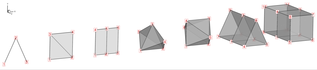
Node numbering (red) for each FE zone type. Node indices are zero-based and are
used directly in the node_map connectivity array passed to
write_fe_zone().#
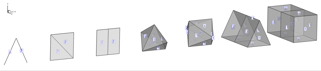
Cell numbering (blue) for each FE zone type. Cell indices correspond to rows
in the node_map array.#
3. Time-Dependent 2-D Field#
Transient datasets are written by assigning each zone a strand_id and
solution_time. Zones on the same strand animate together in Tecplot 360.
Grid coordinates that do not change between time steps can be shared from
the first zone to avoid writing duplicate arrays, which substantially reduces
file size for large grids.
import numpy as np
import tecio

# 2-D grid
nx, ny = 128, 128
x = np.linspace(0.0, 1.0, nx)
y = np.linspace(0.0, 1.0, ny)
X, Y = np.meshgrid(x, y, indexing="ij")  # shape (nx, ny)

times = np.linspace(0.0, 4.0 * np.pi, 60)

with tecio.open("transient.szplt", "w", title="Travelling Wave") as w:
    # Set dataset auxiliary data before the first zone. Because the variable
      indices are the aux data values read by Tepclot, use 1-based indices.
    w.add_auxdataset_dict({
        "Common.XVar": 1,
        "Common.YVar": 2,
        "Common.CVar": 3,
    })

    for i, t in enumerate(times):
        phi = np.sin(2.0 * np.pi * X - t) * np.cos(2.0 * np.pi * Y)

        if i == 0:
            # First zone: write grid coordinates and solution
            w.write_ordered_zone(
                title=f"t = {t:.3f}",
                variables=["x", "y", "phi"],
                data=[X, Y, phi],
                strand_id=1,
                solution_time=t,
            )
        else:
            # Subsequent zones: share x and y from zone 0, write phi only
            w.write_ordered_zone(
                title=f"t = {t:.3f}",
                data=[phi],
                var_sharing={"x": 0, "y": 0},
                strand_id=1,
                solution_time=t,
            )
Reading a transient file works identically to a steady file — the zones are listed in the order they were written:
with tecio.open("transient.szplt", "r") as r:
    print(r.num_zones)  # 60

    # Solution times across all zones
    times_read = [r.zones[i].solution_time for i in range(r.num_zones)]

    # Grid is only stored in zone 0; later zones return None for shared vars
    phi_t0 = r.zones[0].variables[2].values  # shape (128, 128, 1)
    phi_t1 = r.zones[1].variables[2].values  # shape (128, 128, 1)
    x_shared = r.zones[1].variables[0].values  # None — shared from zone 0
4. Low-Level libtecio API#
The tecio.libtecio module exposes the TecIO C functions directly. Using it
gives full control over data types, zone creation options, and the write
ordering required by the SZL API. Unlike the rest of tecio, this module is
a thin ctypes wrapper with no index translation: zone and variable arguments
are passed straight through to TecIO, so they follow TecIO’s own 1-based
convention. This example reproduces the 1-D sine curve from Example 1 using
the low-level SZL write functions.
import numpy as np
from tecio import libtecio
from tecio.libtecio import DataType, FileType, ValueLocation, ZoneType

x = np.linspace(0.0, 2.0 * np.pi, 256, dtype=np.float32)
y = np.sin(x)

# 1. Open a writer handle (returns an opaque C pointer)
handle = libtecio.tec_file_writer_open(
    filename="line_lowlevel.szplt",
    variables=["x", "y"],
    title="Sine Curve (low-level)",
    file_type=FileType.FULL,
)

# 2. Create a zone and get its 1-based index
izone = libtecio.tec_zone_create_ijk(
    handle,
    zone_title="sin(x)",
    imax=256,
    jmax=1,
    kmax=1,
    var_types=[DataType.FLOAT, DataType.FLOAT],
    value_locations=[ValueLocation.NODAL, ValueLocation.NODAL],
)

# 3. Write each variable by 1-based index (zone=1, var=1 / var=2)
libtecio.tec_zone_var_write_float_values(handle, izone, 1, x)
libtecio.tec_zone_var_write_float_values(handle, izone, 2, y.astype(np.float32))

# 4. Close and flush
libtecio.tec_file_writer_close(handle)
Note
SZL vs. classic API. The SZL functions (tec_file_writer_open,
tec_zone_create_ijk, tec_zone_var_write_*) return an explicit file handle
and allow variables to be written in any order after zone creation. Multiple
files can be open simultaneously.
The classic PLT functions (tecini142, teczne142, tecdat142, tecend142)
maintain a single implicit global context: only one file is active at a time
and data must be written in strict zone → variable order. Use the SZL API for
new code unless PLT format is specifically required.
Indexing Conventions#
Context |
Indexing |
Example |
|---|---|---|
Python reader/writer objects ( |
0-based |
|
|
0-based |
|
|
0-based |
|
|
0-based zone number |
|
|
0-based zone number, or |
|
|
0-based node indices |
|
|
0-based, including the face ordinal |
see Writers |
CLI |
0-based |
|
|
1-based, matches TecIO |
|
Tecplot 360 GUI, macro language, and |
1-based, Tecplot’s own convention |
|
|
1-based, so it reads naturally in MATLAB |
|
Everywhere in the Python API, tecio works in zero-based indices, the same
convention as NumPy arrays and Python lists. Two boundaries convert to
Tecplot’s native one-based convention instead, since that’s what the reader on
the other side expects: the raw tecio.libtecio C wrappers and the tec2mat
CLI’s .mat output.
Getting Help#
All public classes and functions have docstrings accessible via Python’s
built-in help() function:
import tecio

help(tecio.open)  # top-level open function
help(tecio.szl.Write)  # SZL writer class and all its methods
help(tecio.libtecio.ZoneType)  # enum values and descriptions
Full API documentation is available in the API Reference,
and runnable demos are provided in the demos/ directory of the repository.